PCA Biplots

suppressPackageStartupMessages(library(bipl5))

This vignette focuses on the modern bipl5 workflow for principal component analysis (PCA) biplots:

init_biplot(...) |> scale_mds(type = "pca", ...)

The mathematical background is the same background documented in wrap_bipl5.PCA(), but the examples below use the newer specification-based workflow because it is the most natural entry point for package users who want to build a single display first and then extend it later.

The goals of this vignette are to:

• construct a PCA biplot with init_biplot() and scale_mds()
• show the printed structure of the resulting bipl5_biplot
• add extra mdsDisplays with append_mdsDisplay()
• demonstrate format_samples() with both one and two categorical stratifications
• explain the PCA fit measures stored in fit_measures
• preserve the current long-form documentation of the PCA biplot mathematics

Building a PCA biplot

init_biplot() stores the data and preprocessing choices, while scale_mds() fits and compiles the requested biplot. If the input data frame contains categorical columns, those columns are retained inside the specification object so they can be used later by format_samples().

iris2 <- iris
iris2$Band <- factor(
  rep(c("class1", "class2", "class3", "class4"), length.out = nrow(iris2))
)

pca_spec <- init_biplot(iris2, scale = TRUE)

bp_pca <- pca_spec |>
  scale_mds(
    type = "pca",
    eigenvectors = c(1, 2),
    group_aes = iris2$Species,
    show_group_means = TRUE
  )

Immediately after scale_mds(), the object contains one compiled display and a PCA fit-measures branch:

bp_pca
#> bipl5_biplot [PCA] 
#> ├── mdsDisplay_12 [PC 1 & 2] <bipl5_mdsDisplay>
#> │   ├── Data <bipl5_data>
#> │   │   ├── sample_coordinates  [150 x 2]
#> │   │   ├── axes_coordinates  [4 axes]
#> │   │   └── translated_axes_coordinates
#> │   ├── trace_data  [35 traces]
#> │   └── annotations  [140 items]
#> └── fit_measures <bipl5_fitmeasures>
#>     ├── CumPred  [5 traces]
#>     ├── CumAd  [4 traces]
#>     ├── VarExp  [5 traces]
#>     ├── Scree  [1 traces]
#>     └── fit_table_12  [PC 1 & 2]

The default PCA plot is interactive. The left-hand side is the biplot itself, while the right-hand side fit panel can be opened from the widget controls.

plot(bp_pca)

Adding more mdsDisplays

The scale_mds() workflow deliberately compiles only the requested pair of principal components. This keeps the initial object light, and it mirrors the fact that a user often wants to start with just one view. Additional views can then be added with append_mdsDisplay().

Here we extend the original PC 1 & 2 display to also include PC 1 & 3 and PC 2 & 3:

bp_pca_full <- bp_pca |>
  append_mdsDisplay(c(1, 3)) |>
  append_mdsDisplay(c(2, 3))

The printed tree now reflects three stored displays and one fit table for each pair:

bp_pca_full
#> bipl5_biplot [PCA] 
#> ├── mdsDisplay_12 [PC 1 & 2] <bipl5_mdsDisplay>
#> │   ├── Data <bipl5_data>
#> │   │   ├── sample_coordinates  [150 x 2]
#> │   │   ├── axes_coordinates  [4 axes]
#> │   │   └── translated_axes_coordinates
#> │   ├── trace_data  [35 traces]
#> │   └── annotations  [140 items]
#> ├── mdsDisplay_13 [PC 1 & 3] <bipl5_mdsDisplay>
#> │   ├── Data <bipl5_data>
#> │   │   ├── sample_coordinates  [150 x 2]
#> │   │   ├── axes_coordinates  [4 axes]
#> │   │   └── translated_axes_coordinates
#> │   ├── trace_data  [35 traces]
#> │   └── annotations  [150 items]
#> ├── mdsDisplay_23 [PC 2 & 3] <bipl5_mdsDisplay>
#> │   ├── Data <bipl5_data>
#> │   │   ├── sample_coordinates  [150 x 2]
#> │   │   ├── axes_coordinates  [4 axes]
#> │   │   └── translated_axes_coordinates
#> │   ├── trace_data  [35 traces]
#> │   └── annotations  [160 items]
#> └── fit_measures <bipl5_fitmeasures>
#>     ├── CumPred  [5 traces]
#>     ├── CumAd  [4 traces]
#>     ├── VarExp  [5 traces]
#>     ├── Scree  [1 traces]
#>     ├── fit_table_12  [PC 1 & 2]
#>     ├── fit_table_13  [PC 1 & 3]
#>     └── fit_table_23  [PC 2 & 3]

The plot now exposes a dropdown for switching between the stored PC pairs.

plot(bp_pca_full)

Formatting samples

format_samples() does not refit the PCA model. It rebuilds the sample-trace block inside each stored mdsDisplay, so it is the right tool when the ordination is fixed but the display grouping needs to change.

We begin with a colour stratification by species:

bp_pca_species <- bp_pca_full |>
  format_samples(
    stratify = "col",
    by = Species,
    col = c("tomato", "steelblue", "darkgreen")
  )

We then add a second categorical stratification through plotting symbols. Since Band is different from Species, the plotted observation traces are rebuilt internally as the observed Species x Band combinations, while the legend is kept readable by showing separate legend sections for the colour and symbol variables.

bp_pca_dual <- bp_pca_species |>
  format_samples(
    stratify = "symbol",
    by = Band,
    pch = c(15, 16, 17, 18)
  )

The formatted object remains a bipl5_biplot, so it can still be printed, subset, extended, and plotted as usual.

plot(bp_pca_dual)

PCA fit measures

PCA biplots are the richest objects in the current package because they carry a full fit_measures branch. The print method makes the available fit objects explicit:

bp_pca_full$fit_measures
#> bipl5_fitmeasures 
#> ├── CumPred  [5 traces]
#> ├── CumAd  [4 traces]
#> ├── VarExp  [5 traces]
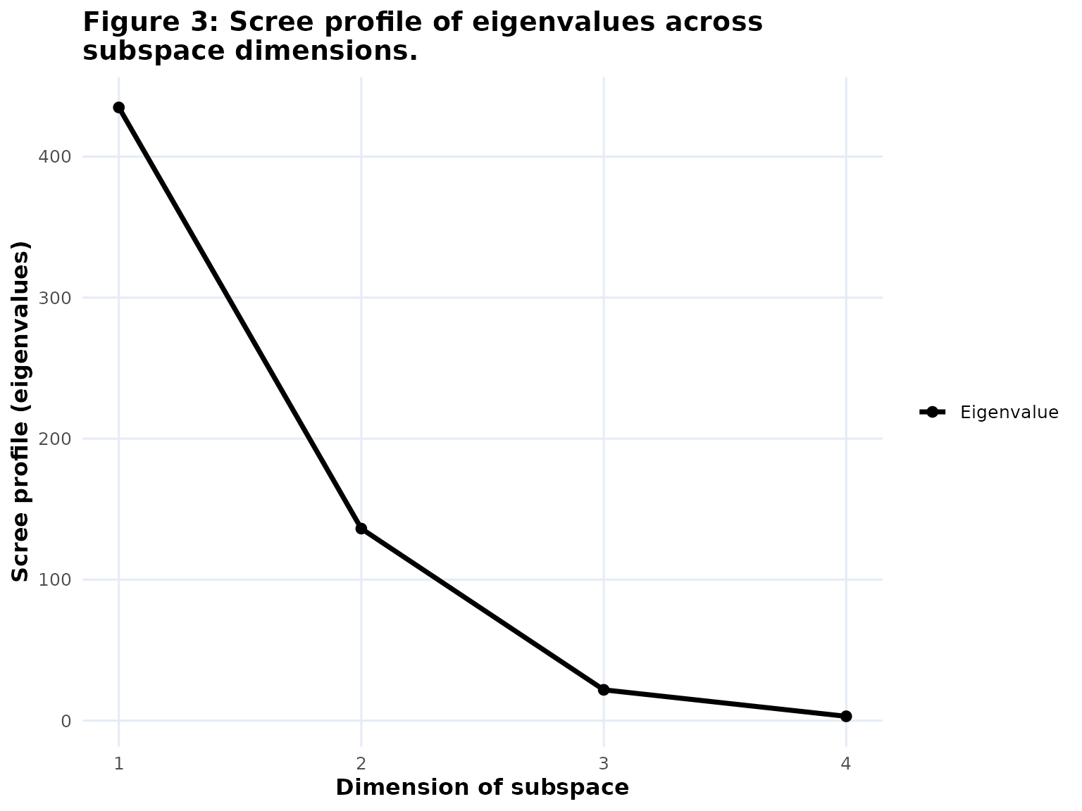
#> ├── Scree  [1 traces]
#> ├── fit_table_12  [PC 1 & 2]
#> ├── fit_table_13  [PC 1 & 3]
#> └── fit_table_23  [PC 2 & 3]

In the interactive PCA widget, these are exposed through the “Measures of Fit” button and the fit-panel dropdown. The fit objects are:

• CumPred: cumulative predictivity across increasing subspace dimension. Each line tracks one variable’s cumulative axis predictivity, and the weighted mean line equals the overall display quality.
• CumAd: cumulative adequacy across increasing subspace dimension. This shows how well each variable direction is represented by the accumulated loading structure, irrespective of the final two-dimensional display pair.
• VarExp: variance explained. In the current implementation this combines a line for the individual proportion of variance explained by each principal component with stacked variable-level contributions.
• Scree: the eigenvalue profile across the principal components.
• fit_table_ij: the pair-specific summary table for the active display. Each table reports variable-level adequacy and predictivity for that specific PC i & j map.

If you want one of the graph-based fit objects on its own, you can extract it and plot it directly:

fit_scree <- extract(bp_pca_full, fit_measures, Scree)
plot(fit_scree)

The summary table is not a separate bipl5_fit graph object, because it is already stored in the fit_measures branch as a plotly table trace. It updates when the active mdsDisplay changes.

Mathematical background

This section preserves the current long-form PCA documentation in narrative form.

Let $\mathbf{X} \in \mathbb{R}^{n \times p}$ denote the processed data matrix stored in the input object after centring and any optional scaling. PCA is performed on that processed matrix, so the singular value decomposition is

$$\mathbf{X} = \mathbf{U}\mathbf{D}\mathbf{V}^{\top},$$

where $\mathbf{U}^{\top}\mathbf{U} = \mathbf{I}$, $\mathbf{V}^{\top}\mathbf{V} = \mathbf{I}$, and $\mathbf{D} = \operatorname{diag}(d_1, \ldots, d_q)$ with $q = \operatorname{rank}(\mathbf{X})$ and $d_1 \ge \cdots \ge d_q \ge 0$. The principal component score vectors are

$$\mathbf{z}_t = d_t \mathbf{u}_t = \mathbf{X}\mathbf{v}_t, \qquad t = 1, \ldots, q.$$

Suppose the displayed pair is $(a, b)$ with $a < b$. Let $\mathbf{J}_{ab}$ be the diagonal selector matrix with ones in positions $a$ and $b$. Then the two-dimensional fitted matrix is

$$\widehat{\mathbf{X}}_{ab} = \mathbf{U}\mathbf{D}\mathbf{J}_{ab}\mathbf{V}^{\top} = \mathbf{X}\mathbf{V}\mathbf{J}_{ab}\mathbf{V}^{\top}.$$

Equivalently, with $\mathbf{U}_{ab}$, $\mathbf{D}_{ab}$, and $\mathbf{V}_{ab}$ containing only the selected components,

$$\widehat{\mathbf{X}}_{ab} = \mathbf{U}_{ab}\mathbf{D}_{ab}\mathbf{V}_{ab}^{\top} = d_a \mathbf{u}_a \mathbf{v}_a^{\top} + d_b \mathbf{u}_b \mathbf{v}_b^{\top}.$$

For the ordinary PCA biplot the displayed sample coordinates are

$$\mathbf{Z}_{ab} = \mathbf{U}_{ab}\mathbf{D}_{ab}, \qquad \mathbf{H}_{ab} = \mathbf{V}_{ab},$$

so that

$$\widehat{\mathbf{X}}_{ab} = \mathbf{Z}_{ab}\mathbf{H}_{ab}^{\top}.$$

If $\mathbf{h}_{(j)}$ is the displayed direction for variable $j$, then the fitted value for observation $i$ on variable $j$ is

$$\widehat{x}_{ij} = \mathbf{z}_i^{\top}\mathbf{h}_{(j)},$$

and the calibrated axis point corresponding to marker value $\mu$ is

$$\mathbf{p}_{\mu j} = \frac{\mu}{\mathbf{h}_{(j)}^{\top}\mathbf{h}_{(j)}}\mathbf{h}_{(j)}.$$

For a correlation biplot the factorization can instead be written as

$$\widehat{\mathbf{X}}_{ab} = \mathbf{U}_{ab}(\mathbf{V}_{ab}\mathbf{D}_{ab})^{\top},$$

so the displayed sample coordinates are $\mathbf{U}_{ab}$ and the displayed variable directions are the rows of $\mathbf{V}_{ab}\mathbf{D}_{ab}$. In that setting the variable directions are tuned to variable-correlation structure rather than raw score geometry.

Two orthogonality relations are central:

$$\mathbf{X}\mathbf{X}^{\top} = \widehat{\mathbf{X}}_{ab}\widehat{\mathbf{X}}_{ab}^{\top} + \mathbf{E}_{ab}\mathbf{E}_{ab}^{\top},$$

and

$$\mathbf{X}^{\top}\mathbf{X} = \widehat{\mathbf{X}}_{ab}^{\top}\widehat{\mathbf{X}}_{ab} + \mathbf{E}_{ab}^{\top}\mathbf{E}_{ab},$$

where $\mathbf{E}_{ab} = \mathbf{X} - \widehat{\mathbf{X}}_{ab}$. The first justifies sample-side fit measures (Type A orthogonality), and the second justifies variable-side fit measures (Type B orthogonality).

For sample $i$, the sample predictivity is

$$\psi_i = \frac{\|\widehat{\mathbf{x}}_{i\cdot}\|^2} {\|\mathbf{x}_{i\cdot}\|^2} = 1 - \frac{\|\mathbf{x}_{i\cdot} - \widehat{\mathbf{x}}_{i\cdot}\|^2} {\|\mathbf{x}_{i\cdot}\|^2}.$$

For variable $j$, the axis predictivity is

$$\phi_j = \frac{\|\widehat{\mathbf{x}}_{(j)}\|^2} {\|\mathbf{x}_{(j)}\|^2} = 1 - \frac{\|\mathbf{x}_{(j)} - \widehat{\mathbf{x}}_{(j)}\|^2} {\|\mathbf{x}_{(j)}\|^2}.$$

The overall quality of the displayed PCA plane is

$$R^2_{\mathrm{disp},ab} = \frac{\|\widehat{\mathbf{X}}_{ab}\|_F^2}{\|\mathbf{X}\|_F^2} = \frac{d_a^2 + d_b^2}{\sum_{t = 1}^q d_t^2}.$$

Because of orthogonality, this same quantity can be read as a weighted average of either the sample predictivities or the axis predictivities. On the variable side,

$$R^2_{\mathrm{disp},ab} = \sum_{j = 1}^p w_j \phi_j, \qquad w_j = \frac{\|\mathbf{x}_{(j)}\|^2}{\|\mathbf{X}\|_F^2}.$$

When the processed variables all have equal sums of squares, the overall quality is simply the average axis predictivity. This is one reason standardized PCA is often easy to interpret.

PCA also gives a clean per-component decomposition. Since

$$\widehat{\mathbf{X}}_{ab} = d_a \mathbf{u}_a \mathbf{v}_a^{\top} + d_b \mathbf{u}_b \mathbf{v}_b^{\top},$$

the two displayed rank-1 pieces are orthogonal, and therefore

$$R^2_{\mathrm{disp},ab} = R_a^2 + R_b^2, \qquad R_a^2 = \frac{d_a^2}{\|\mathbf{X}\|_F^2}, \qquad R_b^2 = \frac{d_b^2}{\|\mathbf{X}\|_F^2}.$$

Likewise,

$$\phi_j = \phi_{ja} + \phi_{jb}, \qquad \psi_i = \psi_{ia} + \psi_{ib},$$

so both axis-side and sample-side quality can be broken down into the two displayed components.

The package documentation also distinguishes these sum-of-squares measures from the direct-reading diagnostics of Alves (2012). If $\mathbf{g}_{(j)}$ is the displayed direction of variable $j$, then the read-off value on that axis for sample $i$ is

$$\widehat{x}_{ij} = \mathbf{z}_i^{\top}\mathbf{g}_{(j)}.$$

The direct-reading error is

$$\delta_{ij} = \frac{|x_{ij} - \widehat{x}_{ij}|}{s_j},$$

where $s_j$ is the standard deviation used in preprocessing, and the mean axis-level direct-reading error is

$$\bar{\delta}_j = \frac{1}{n}\sum_{i = 1}^n \delta_{ij}.$$

These quantities answer a different question from predictivity. Predictivity asks how much sum of squares is reproduced by the displayed plane. The Alves diagnostics ask how accurately values can be read directly from the plotted calibrated axes.

References

Alves, M. R. (2012). Evaluation of the predictive power of biplot axes to automate the construction and layout of biplots based on the accuracy of direct readings from common outputs of multivariate analyses: application to principal component analysis. Journal of Chemometrics, 26(5), 180-190.

Eckart, C. and Young, G. (1936). The approximation of one matrix by another of lower rank. Psychometrika, 1, 211-218.

Gabriel, K. R. (1971). The biplot graphical display of matrices with application to principal component analysis. Biometrika, 58(3), 453-467.

Gardner-Lubbe, S., le Roux, N. J. and Gower, J. C. (2008). Measures of fit in principal component and canonical variate analyses. Journal of Applied Statistics, 35(9), 947-965.

Gower, J. C. and Hand, D. J. (1996). Biplots. London: Chapman and Hall.

Gower, J. C., Lubbe, S. and le Roux, N. J. (2011). Understanding Biplots. Chichester: Wiley.

Greenacre, M. (2010). Biplots in Practice. Bilbao: BBVA Foundation.